Drake Introduction 1 - Bringing An Object Into the World

May 25 2022

(This is Part 1 of a planned series of posts on the robotic simulation library Drake developed by MIT and TRI. Part 2 is here.)

Objective

The goal of this article is to give an example of some useful concepts of Drake, specifically:

• Diagrams
• Multibody Systems
• Pose of Rigid Bodies

We will do this by creating a Python program that will drop a block into an empty scene and then save the trajectory that it undergoes. (For more information, feel free to visit the Drake's Python Documentation or working libraries like kinova_drake.)

Getting Your Object

The first example we will investigate is about inserting an object into a scene and simulating what it does.

To do this, we will first need an object model (in this case a .urdf file) as well as a representation of the ground in our world.

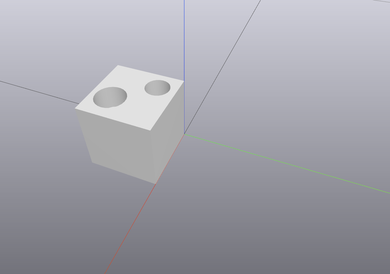
The object that we will insert into this scene is this simple cube with two curious holes molded into its top.

The block above was made in a 3D drawing program (Autodesk Fusion 360). It is typically saved as an .stl file. See the appendix below for how to convert this into a .urdf file.

Starting Your Diagram

Next, let us sketch out a view of all of the parts that we want to exist in our simulation.

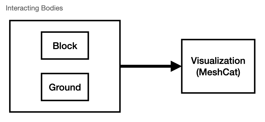
In this diagram we simply want to place a block into a world with a 'floor'. We only need the block and the floor to be interacting bodies here.

The way that drake will work is that we will assemble these parts into a Diagram. The object that assembles our Diagram's components is the DiagramBuilder:

builder = DiagramBuilder()

Next, let's create the interacting bodies. These will be represented as a Multibody in Drake's parlance. To create it, we will type the following lines:

        
plant, scene_graph = AddMultibodyPlantSceneGraph(builder, time_step=1e-3)
block_as_model = Parser(plant=plant).AddModelFromFile(
    "/root/OzayGroupExploration/drake/manip_tests/slider/slider-block.urdf",
    'block_with_slots')
AddGround(plant)
        
    

The first line in the above list adds both a new Multibody plant and a new SceneGraph (for Visualization) to the diagram and then connects them. The second line adds a specific model to the plant, it is the model stored at the directory given in the first string input to AddModelFromFile(). And the third line adds a plane to the world with certain friction coefficients via a homemade function called AddGround(). See Appendix B below to learn more.

From here, we will finalize the plant (plant.Finalize()) which is necessary if we want to begin connecting some of its ports to other objects in our diagram. We will then add an additional useful element to our diagram, it is a logger:

Monitoring the Block's Trajectory

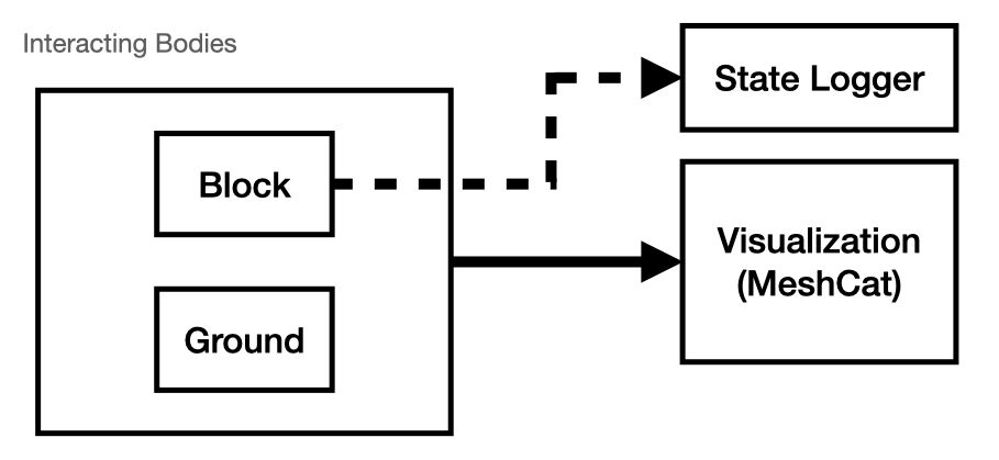
We would like to save the trajectory data of the cube. So, we need an additional component: A Logger.

What we want to do is to connect the state of the block to this logger so that we can collect the data of it bouncing on the floor during simulation. To do this we add the following lines to our python script:

        
state_logger = LogVectorOutput(plant.get_state_output_port(block_as_model), builder)
state_logger.set_name("state_logger")
        
    

We also name the log with a predictable name. Finally, we connect the scene graph to a Meshcat server. Simply put, this makes it so that the 3D bodies that we defined are visible through the Meshcat viewer (basically a webpage that will become available on your local computer). I will not discuss much of what Meshcat is, but you can read more by clicking here.

        
meshcat = ConnectMeshcatVisualizer(builder=builder,
    zmq_url = zmq_url,
    scene_graph=scene_graph,
    output_port=scene_graph.get_query_output_port())
        
    

Congratulations! With all of this code you have completely defined our desired block diagram! You can now add the line builder.Build() to the script and it will assemble all of these elements together.

Defining the Block's Initial State

To make the simulation more interesting, I will control the initial pose of the block in the scene using the following code:

        
diagram_context = diagram.CreateDefaultContext()
p_WBlock = [0.0, 0.0, 0.1]
R_WBlock = RotationMatrix.MakeXRotation(np.pi/2.0)
X_WBlock = RigidTransform(R_WBlock,p_WBlock)
plant.SetFreeBodyPose(
    plant.GetMyContextFromRoot(diagram_context),
    plant.GetBodyByName("body", block_as_model),
    X_WBlock)
plant.SetFreeBodySpatialVelocity(
    plant.GetBodyByName("body", block_as_model),
    SpatialVelocity(np.zeros(3),np.array([0.0,0.0,0.0])),
    plant.GetMyContextFromRoot(diagram_context))

meshcat.load()
diagram.Publish(diagram_context)
        
    

These lines are doing a lot, but they are simply stating that they want to make the initial state of the block have a certain pose (or RigidBodyTransform) which is X_WBlock. The next lines then force the block to start with that pose and zero velocity. So that the block falls from rest. The other lines in this sequence simply start the meshcat server and connect the diagram to it.

Running Your Simulation

        
# Set up simulation
simulator = Simulator(diagram, diagram_context)
simulator.set_target_realtime_rate(1.0)
simulator.set_publish_every_time_step(False)

# Run simulation
simulator.Initialize()
simulator.AdvanceTo(15.0)
        
    

These lines are a bit more straight forward. We create a simulator associated with this diagram and the current diagram context along with a realtime rate of 1.0 and other flags. Then the simulator is started and we advance it 15 seconds. If you would like to view the trajectory data of the block, then you can add the following lines:

        
# Collect Data
state_log = state_logger.FindLog(diagram_context)
log_times  = state_log.sample_times()
state_data = state_log.data()
print(state_data.shape)
        
    

What you will discover is that log_times and state_data are numpy arrays. You can do all of the plotting or other manipulations that you might normally use on your numpy arrays on that data, including plotting.

See the file slider_init.py which contains all of the elements discussed above and more.

--

Appendix 1: .STL to .URDF

The first step in the conversion process is to use a tool like Fusion 360 to save/export the .STL file into an .OBJ file. (If there are multiple parts, then you may want to save the .STL file into multiple individual .OBJ files.)

Once saved as an .obj file, I created a "robot" in a urdf file and gave it a single "link" which I called body. The inertial parameters (mass, moment of inertia, etc.), its visual parameters (mainly the geometry from the .obj) and its collision properties (again the geometry that describes how it comes into contact with the world) can all be defined once the .obj is available. See this .urdf file for an example of how to do this.

Note: For whatever reason, in the conversion from .stl to .obj, the units defining the dimensions tend to get messed up. You may need to use the "scale" tag in order to correct for this unanticipated scaling.

Appendix 2: AddGround()

The code contained within AddGround() is as follows:

        
def AddGround(plant):
    """
    Add a flat ground with friction
    """

    # Constants
    transparent_color = np.array([0.5,0.5,0.5,0])
    nontransparent_color = np.array([0.5,0.5,0.5,0.1])

    p_GroundOrigin = [0, 0.0, 0.0]
    R_GroundOrigin = RotationMatrix.MakeXRotation(0.0)
    X_GroundOrigin = RigidTransform(R_GroundOrigin,p_GroundOrigin)

    # Set Up Ground on Plant

    surface_friction = CoulombFriction(
            static_friction = 0.7,
            dynamic_friction = 0.5)
    plant.RegisterCollisionGeometry(
            plant.world_body(),
            X_GroundOrigin,
            HalfSpace(),
            "ground_collision",
            surface_friction)
    plant.RegisterVisualGeometry(
            plant.world_body(),
            X_GroundOrigin,
            HalfSpace(),
            "ground_visual",
            transparent_color)  # transparent
        
    

Importantly, this code shows that you can insert objects into Drake by importing .urdf files OR by creating them with some of the functions built into Drake. Note that in this function, we create the desired color of the plane and where it's located in the world (in this case at the origin with its axes aligned to the world axes). We then define the friction characteristics and use all of the variables created above to define:

• Adds a new body to the current plant (plant is the object calling the RegisterCollisionGeometry() function),
• Registers the new collision geometry to the world_body() of our plant,
• Fixes the pose of the new "ground plane" to be located at the pose X_GroundOrigin with respect to the origin of world_body()'s frame,
• Defines the shape of the "ground" to be a HalfSpace(),
• Gives the "ground" the desired surface properties.

See the documentation for RegisterCollisionGeometry() for more details.

Similarly, this code also defines the visual geometry (or what we see through MeshCat) through a similar function. See the documentation for RegisterCollisionGeometry() for more details.